
PyFrag 2019
See documentation for tutorials and documentation.
NOTICE(October 28 2021)
Since ADF2019, the ADF has been reconfigured and renamed as AMS2020 and AMS2021. Accordingly the format of input has also changed a lot. PyFrag has now been updated as well to be compatible with these changes. Old users can delete old version and reinstall the new version. If user still chooses ADF2019 or older version of ADF as the computational engine, one can use the command pyfrag -x adfold job.in to invoke PyFrag.
Motivation
The PyFrag 2019 program was specially designed to facilitate the analysis of reaction mechanism in a more efficient and user-friendly way. The original PyFrag 2008 workflow facilitated the characterization of reaction mechanisms in terms of the intrinsic properties, such as strain and interaction, of the reactants. This approach is routinely applied in the Bickelhaupt Group to understand numerous organic, inorganic, and biomolecular reactions/processes. The new PyFrag 2019 program has automated and reduced the time-consuming and laborious task of setting up, running, analyzing, and visualizing computational data from reaction mechanism studies to a single job. PyFrag 2019 resolves three main challenges associated with the automatized computational exploration of reaction mechanisms: 1) the management of multiple parallel calculations to automatically find a reaction path; 2) the monitoring of the entire computational process along with the extraction and plotting of relevant information from large amounts of data; and 3) the analysis and presentation of these data in a clear and informative way. The activation strain and canonical energy decomposition results that are generated, relate the characteristics of the reaction profile in terms of intrinsic properties (strain, interaction, orbital overlaps, orbital energies, populations) of the reactant species.
Description
Usage
In order to see all the commands that can be used in this program, the user can type pyfrag -h, which will show:
Usage: pyfrag [-h] [-s] [-x command]  [...]
-h          : print this information
-s          : run job quietly
-x          : start the executable named command
            : command include restart, which restart job
            : restart, which restart a job after it is stoped
            : summary, which summarize all job result after jobs finished
            : default command is pyfrag itself
The example command is like as follow, in which job.in is job input
pyfrag job.in
or
pyfrag -x restart job.in
or
pyfrag -s -x summary job.in
Input example
A simple job input is provided below. The input script can be roughly divided into four section: the required submit information for a job scheduling system (Slurm in this example), ADF parameters, pyfrag parameters, and geometry parameters. Additional information about the input file can be found in input explanation and main specifications in the following webpages.
JOBSUB
#!/bin/bash
#SBATCH -J frag_1
#SBATCH -N 1
#SBATCH -t 50:00
#SBATCH --ntasks-per-node=24
#SBATCH --partition=short
#SBATCH --output=%job.stdout
#SBATCH --error=%job.stdout
export NSCM=24

JOBSUB END

ADF

basis
type TZ2P
core Small
end

xc
gga OPBE
end

relativistic SCALAR ZORA

scf
iterations 299
converge 0.00001
mixing 0.20
end

numericalquality verygood

charge 0 0
symmetry auto

ADF END

PyFrag

fragment  2
fragment  1 3 4 5 6
strain    0
strain   -554.09
bondlength 1 6  1.09

PyFrag END

Geometrycoor

R1: Fe-II(CO)4 + CH4
Pd       0.00000000       0.00000000       0.32205546

R2: CH4
C       0.00000000       0.00000000      -1.93543634
H      -0.96181082       0.00000000      -1.33610429
H       0.00000000      -0.90063254      -2.55201285
H       0.00000000       0.90063254      -2.55201285
H       0.96181082       0.00000000      -1.33610429

RC: Fe-II(CO)4 + CH4
C       0.00000000       0.00000000      -1.93543615
Pd       0.00000000       0.00000000       0.322055
H      -0.96181082       0.00000000      -1.33610429
H       0.00000000      -0.90063254      -2.55201285
H       0.00000000       0.90063254      -2.55201285
H       0.96181082       0.00000000      -1.33610429

TS: Fe-II(CO)4 + CH4
C      -1.74196777      -2.22087997       0.00000000
Pd     -2.13750904      -0.23784341       0.00000000
H      -2.80956968      -2.49954731       0.00000000
H      -1.26528821      -2.62993236       0.8956767
H      -1.26528821      -2.62993236      -0.895676
H      -0.75509932      -0.88569836       0.00000000

P: Fe-II(CO)4 + CH4
C      -2.10134690      -2.41901732       0.1862099
Pd      -2.73145901      -0.57025833       0.419766
H      -3.88639130      -1.04648079      -0.43099501
H      -2.78392696      -3.12497645       0.66994616
H      -1.97386865      -2.66955518      -0.87144525
H      -1.12556673      -2.41201402       0.698583

Geometrycoor END
Result example
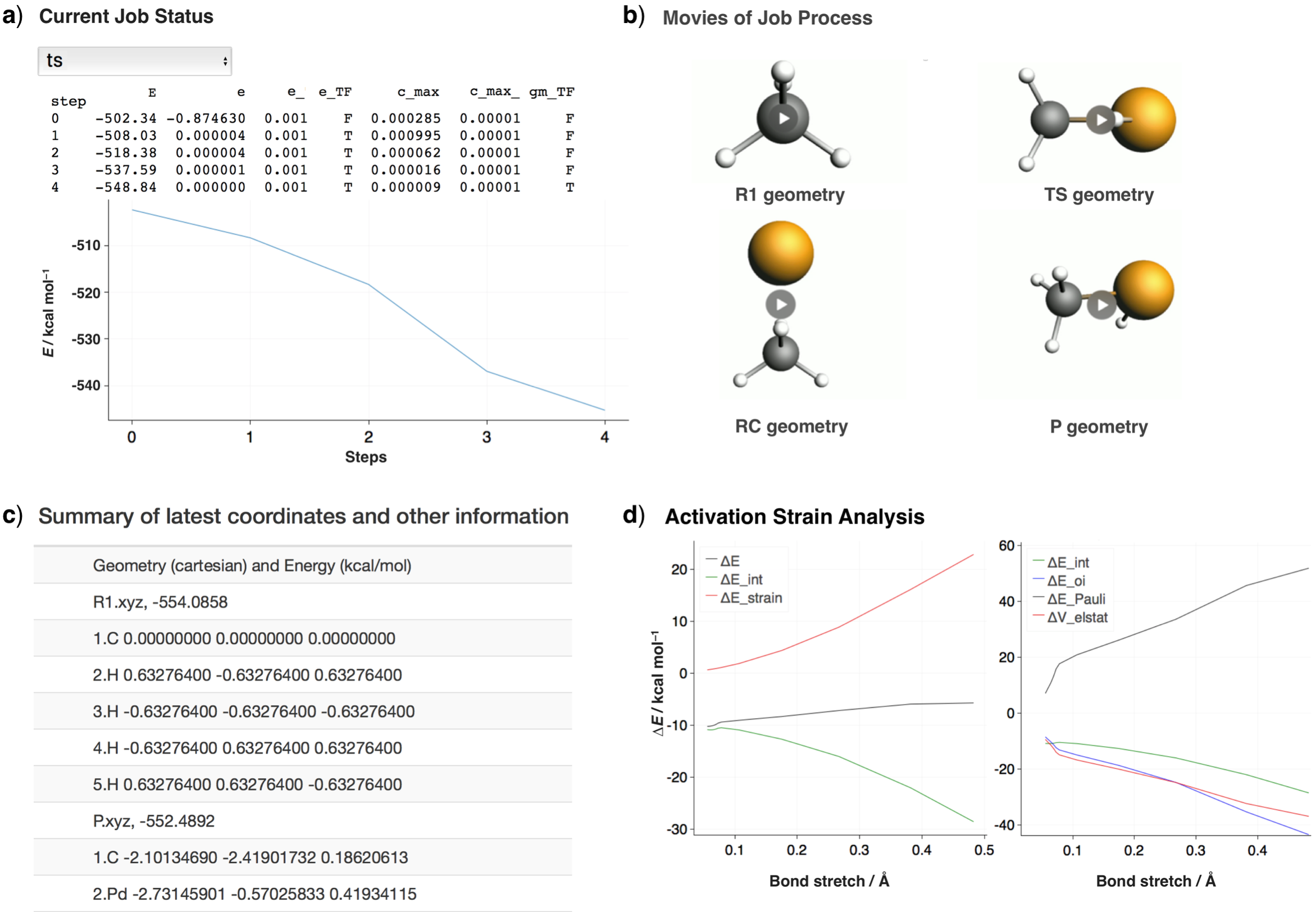
After the job has been submitted, a website as provided in the figure below will be launched that summarizes all relevant information, including: a) the convergence information, b) the latest structure from the optimization in the form of movie, c) the latest energy and coordinates, and d) the activation strain analysis (if a job is finished). The user can decide if the trend of optimization is right or wrong, and if necessary, the job can be stopped. If the input file has been modified, the job will be resubmitted and the overall workflow will resume from where it stopped before.
Installation
For installation, please read installation.